intNMF examples
Load required libraries. int_nmf_model must be in the same directory. If it is not it can be added to pythons path
[10]:
import anndata as ad
import scanpy as sc
import numpy as np
import scipy
from scripts.int_nmf_model import intNMF, log_tf_idf
import anndata as ad
from matplotlib import pyplot as plt
import scipy.io
import pandas as pd
This notebook contains some examples of what intNMF can do including how to load multiome data stored as three different file types.
Example 1 - anndata
Probably the simplest case where the multiome data is stored as anndata object. https://anndata.readthedocs.io/en/latest/. Dataset from recent neurips competition
Add file locations and load the data
[11]:
atac_loc = 'data/anndata/openproblems_bmmc_multiome_phase2.censor_dataset.output_mod1.h5ad'  #comp data multi
rna_loc = 'data/anndata/openproblems_bmmc_multiome_phase2.censor_dataset.output_mod2.h5ad'
res_loc = 'data/anndata/openproblems_bmmc_multiome_phase2.censor_dataset.output_solution.h5ad'
[12]:
res
[12]:
'data/anndata/openproblems_bmmc_multiome_phase2.censor_dataset.output_solution.h5ad'
[13]:
atac_mat = ad.read_h5ad(atac_loc)
rna_mat = ad.read_h5ad(rna_loc)
[14]:
res_mat = ad.read_h5ad(res_loc)
[15]:
res_mat
[15]:
AnnData object with n_obs × n_vars = 42492 × 13431
    obs: 'batch', 'cell_type', 'pseudotime_order_GEX', 'pseudotime_order_ATAC'
    var: 'gene_ids', 'feature_types'
    uns: 'dataset_id', 'organism'
[16]:
atac_mat.obs['cell_type'] = res_mat.obs['cell_type']
In this case the atac data is binary and the rna data are real numbers. This data has already been preprocessed and filtered. Before carrying out the matrix factorisation log_tf_idf transform the data
[17]:
atac_mat_tfidf_log = log_tf_idf(atac_mat.X)
rna_mat_tfidf_log = log_tf_idf(rna_mat.X)
initialise the nmf model then fit the model. This minimises the error X - WH for the atac and rna matrices respectively
[18]:
nmf_model = intNMF(20, epochs = 20, init = 'random')
nmf_model.fit(rna_mat_tfidf_log, atac_mat_tfidf_log)
Theta holds the topic activities in each cell. Numpy array of shape cell x topic
[19]:
nmf_model.theta.shape
[19]:
(42492, 20)
phi rna and phi atac hold the topic loadings or ‘definitions’ which facilitate recontruction of X from the latent topics. Numpy array of shape topic x feature (e.g. accessible chromatin or gene expression)
[20]:
print(nmf_model.phi_rna.shape)
nmf_model.phi_atac.shape
(20, 116490)
[20]:
(20, 13431)
Example plots to view the NMF matrices
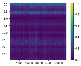
View topic x gene matrix. These matrices have been thresholded at one to improve visualisation
[21]:
plt.imshow(np.where(nmf_model.phi_rna > 1, 1, nmf_model.phi_rna), aspect=nmf_model.phi_rna.shape[1]/nmf_model.phi_rna.shape[0], interpolation=None)
cbar = plt.colorbar()
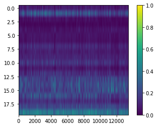
View topic x peak matrix.
[22]:
plt.imshow(np.where(nmf_model.phi_atac > 1, 1, nmf_model.phi_atac), aspect=nmf_model.phi_atac.shape[1]/nmf_model.phi_atac.shape[0], interpolation=None)
cbar = plt.colorbar()
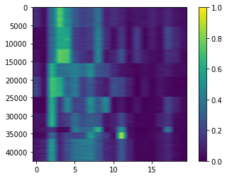
View cell x topic matrix
[23]:
plt.imshow(np.where(nmf_model.theta > 1, 1, nmf_model.theta), aspect=nmf_model.theta.shape[1]/nmf_model.theta.shape[0], interpolation=None)
cbar = plt.colorbar()
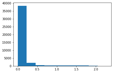
Plots to view histograms of individual topics or whole matrices.
Whole matrix
[24]:
plt.hist(nmf_model.theta.ravel())
[24]:
(array([8.14293e+05, 2.89050e+04, 3.71900e+03, 1.12200e+03, 7.99000e+02,
        6.88000e+02, 2.22000e+02, 5.70000e+01, 2.20000e+01, 1.30000e+01]),
 array([1.25888058e-15, 1.25888058e+00, 2.51776115e+00, 3.77664173e+00,
        5.03552231e+00, 6.29440288e+00, 7.55328346e+00, 8.81216404e+00,
        1.00710446e+01, 1.13299252e+01, 1.25888058e+01]),
 <BarContainer object of 10 artists>)

Just the first topic
[25]:
plt.hist(nmf_model.theta[:, 0].ravel())
[25]:
(array([3.8342e+04, 1.9830e+03, 4.9800e+02, 2.7700e+02, 2.8300e+02,
        3.8400e+02, 3.9600e+02, 2.4500e+02, 7.3000e+01, 1.1000e+01]),
 array([1.27215510e-15, 2.27702815e-01, 4.55405629e-01, 6.83108444e-01,
        9.10811259e-01, 1.13851407e+00, 1.36621689e+00, 1.59391970e+00,
        1.82162252e+00, 2.04932533e+00, 2.27702815e+00]),
 <BarContainer object of 10 artists>)
Or the gene contributions to the first topic
[26]:
plt.hist(nmf_model.phi_rna[0, :].ravel())
[26]:
(array([8.5861e+04, 1.9619e+04, 7.0380e+03, 2.5430e+03, 9.1300e+02,
        3.3200e+02, 1.2300e+02, 3.4000e+01, 2.2000e+01, 5.0000e+00]),
 array([7.91979667e-16, 5.09246303e-01, 1.01849261e+00, 1.52773891e+00,
        2.03698521e+00, 2.54623152e+00, 3.05547782e+00, 3.56472412e+00,
        4.07397042e+00, 4.58321673e+00, 5.09246303e+00]),
 <BarContainer object of 10 artists>)

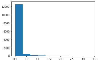
Or the chromtin peak contributions to the first topic
[27]:
plt.hist(nmf_model.phi_atac[0, :].ravel())
[27]:
(array([1.2585e+04, 4.5900e+02, 1.5500e+02, 8.7000e+01, 4.1000e+01,
        4.4000e+01, 3.1000e+01, 1.7000e+01, 7.0000e+00, 5.0000e+00]),
 array([1.07812024e-15, 3.34391016e-01, 6.68782032e-01, 1.00317305e+00,
        1.33756406e+00, 1.67195508e+00, 2.00634610e+00, 2.34073711e+00,
        2.67512813e+00, 3.00951914e+00, 3.34391016e+00]),
 <BarContainer object of 10 artists>)
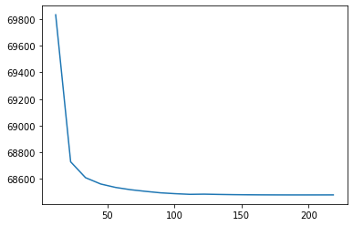
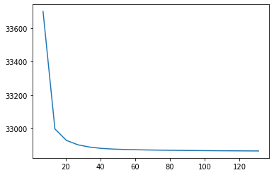
Plot to view loss over time
[28]:
fig, ax = plt.subplots()

ax.plot(np.cumsum(nmf_model.epoch_times), nmf_model.loss)
[28]:
[<matplotlib.lines.Line2D at 0x7f8140541970>]
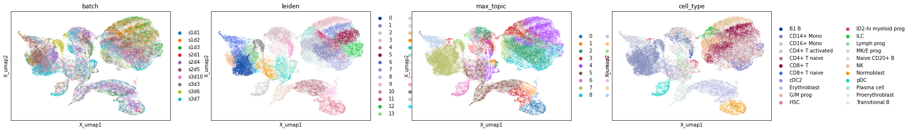
Using Scanpys plotting methods
For this dataset there are ground truth labels (although I think I’ve got a version without cell labels here). Below is an example of how to visualise the NMF embedding of the data using UMAP. This closely mirrors this tutorial https://scanpy-tutorials.readthedocs.io/en/latest/pbmc3k.html.
[29]:
atac_mat.obsm['nmf'] = nmf_model.theta
rna_mat.obsm['nmf'] = nmf_model.theta
[30]:
atac_mat
[30]:
AnnData object with n_obs × n_vars = 42492 × 13431
    obs: 'batch', 'size_factors', 'cell_type'
    var: 'gene_ids', 'feature_types'
    uns: 'dataset_id', 'organism'
    obsm: 'nmf'
    layers: 'counts'
[31]:
sc.pp.neighbors(atac_mat, use_rep='nmf', n_pcs=100)
sc.tl.umap(atac_mat)
sc.tl.leiden(atac_mat)
[32]:
atac_mat.obs['max_topic'] = np.argmax(atac_mat.obsm['nmf'], axis=1)
atac_mat.obs['max_topic']  = atac_mat.obs['max_topic'].astype("category")
[33]:
sc.pl.embedding(atac_mat, 'X_umap', color=['batch', 'leiden', 'max_topic', 'cell_type'])
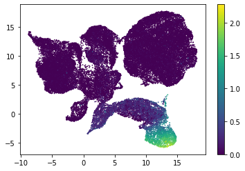
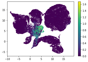
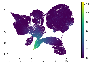
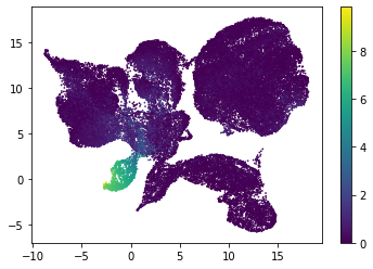
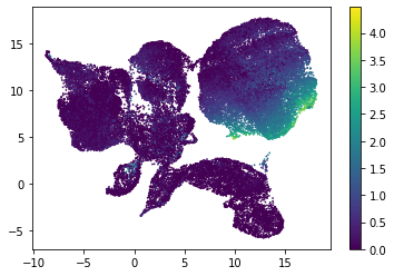
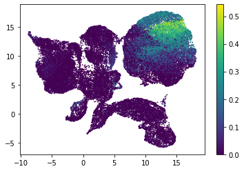
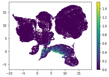
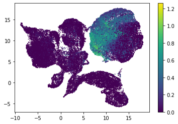
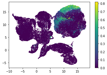
[34]:
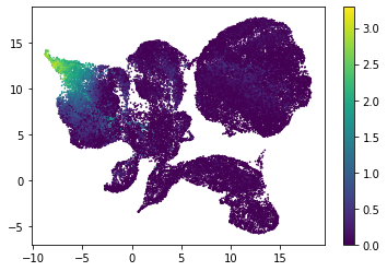
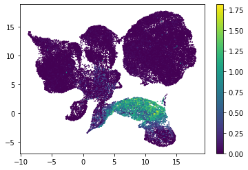
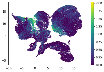
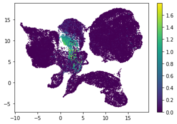
for i in range(atac_mat.obsm['nmf'].shape[1]):
    plt.scatter(atac_mat.obsm['X_umap'][:, 0], atac_mat.obsm['X_umap'][:, 1], c=atac_mat.obsm['nmf'][:, i], s=0.5)
    plt.colorbar()
    plt.show()


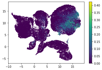
Or use PCA embedding to visualise topic scores
[35]:
sc.tl.pca(atac_mat, svd_solver='arpack')
sc.pp.neighbors(atac_mat, n_neighbors=50, n_pcs=100, use_rep='X_pca', key_added='pca_nb')
sc.tl.umap(atac_mat, neighbors_key='pca_nb')
[36]:
sc.pl.embedding(atac_mat, 'X_umap', color=['batch', 'leiden', 'max_topic', 'cell_type'])

Example 2 - 10x HDF5 data
10x data pbmc 10k sorted. HDF5 https://support.10xgenomics.com/single-cell-multiome-atac-gex/software/pipelines/latest/advanced/h5_matrices
[37]:
import collections
import scipy.sparse as sp_sparse
import tables
import scanpy as sc
CountMatrix = collections.namedtuple('CountMatrix', ['feature_ref', 'barcodes', 'matrix'])
function from above link
[38]:
def get_matrix_from_h5(filename):
    with tables.open_file(filename, 'r') as f:
        mat_group = f.get_node(f.root, 'matrix')
        barcodes = f.get_node(mat_group, 'barcodes').read()
        data = getattr(mat_group, 'data').read()
        indices = getattr(mat_group, 'indices').read()
        indptr = getattr(mat_group, 'indptr').read()
        shape = getattr(mat_group, 'shape').read()
        matrix = sp_sparse.csc_matrix((data, indices, indptr), shape=shape)

        feature_ref = {}
        feature_group = f.get_node(mat_group, 'features')
        feature_ids = getattr(feature_group, 'id').read()
        feature_names = getattr(feature_group, 'name').read()
        feature_types = getattr(feature_group, 'feature_type').read()
        feature_ref['id'] = feature_ids
        feature_ref['name'] = feature_names
        feature_ref['feature_type'] = feature_types
        tag_keys = [key.decode() for key in getattr(feature_group, '_all_tag_keys').read()]
        for key in tag_keys:
            feature_ref[key] = getattr(feature_group, key).read()

        return CountMatrix(feature_ref, barcodes, matrix)
[39]:
filtered_matrix_h5 = "data/10x/hdf5/pbmc_granulocyte_sorted_10k_filtered_feature_bc_matrix.h5"
filtered_feature_bc_matrix = get_matrix_from_h5(filtered_matrix_h5)
[40]:
filtered_feature_bc_matrix[0]
[40]:
{'id': array([b'ENSG00000243485', b'ENSG00000237613', b'ENSG00000186092', ...,
        b'KI270713.1:29624-30457', b'KI270713.1:31340-32243',
        b'KI270713.1:36927-37836'], dtype='|S26'),
 'name': array([b'MIR1302-2HG', b'FAM138A', b'OR4F5', ...,
        b'KI270713.1:29624-30457', b'KI270713.1:31340-32243',
        b'KI270713.1:36927-37836'], dtype='|S26'),
 'feature_type': array([b'Gene Expression', b'Gene Expression', b'Gene Expression', ...,
        b'Peaks', b'Peaks', b'Peaks'], dtype='|S15'),
 'genome': array([b'GRCh38', b'GRCh38', b'GRCh38', ..., b'GRCh38', b'GRCh38',
        b'GRCh38'], dtype='|S6'),
 'interval': array([b'chr1:29553-30267', b'chr1:36080-36081', b'chr1:65418-69055', ...,
        b'KI270713.1:29624-30457', b'KI270713.1:31340-32243',
        b'KI270713.1:36927-37836'], dtype='|S26')}
[41]:
filtered_feature_bc_matrix[1]
[41]:
array([b'AAACAGCCAAGGAATC-1', b'AAACAGCCAATCCCTT-1',
       b'AAACAGCCAATGCGCT-1', ..., b'TTTGTTGGTTGCAGTA-1',
       b'TTTGTTGGTTGGTTAG-1', b'TTTGTTGGTTTGCAGA-1'], dtype='|S18')
[42]:
filtered_feature_bc_matrix[2]
[42]:
<180488x11898 sparse matrix of type '<class 'numpy.int32'>'
        with 127525374 stored elements in Compressed Sparse Column format>
[43]:
multi_10x = ad.AnnData( filtered_feature_bc_matrix[2].T,
                        filtered_feature_bc_matrix[1],
                        filtered_feature_bc_matrix[0])
[44]:
multi_10x.var
[44]:
| id | name | feature_type | genome | interval | |
|---|---|---|---|---|---|
| 0 | b'ENSG00000243485' | b'MIR1302-2HG' | b'Gene Expression' | b'GRCh38' | b'chr1:29553-30267' |
| 1 | b'ENSG00000237613' | b'FAM138A' | b'Gene Expression' | b'GRCh38' | b'chr1:36080-36081' |
| 2 | b'ENSG00000186092' | b'OR4F5' | b'Gene Expression' | b'GRCh38' | b'chr1:65418-69055' |
| 3 | b'ENSG00000238009' | b'AL627309.1' | b'Gene Expression' | b'GRCh38' | b'chr1:120931-133723' |
| 4 | b'ENSG00000239945' | b'AL627309.3' | b'Gene Expression' | b'GRCh38' | b'chr1:91104-91105' |
| ... | ... | ... | ... | ... | ... |
| 180483 | b'KI270713.1:21434-22340' | b'KI270713.1:21434-22340' | b'Peaks' | b'GRCh38' | b'KI270713.1:21434-22340' |
| 180484 | b'KI270713.1:26201-26826' | b'KI270713.1:26201-26826' | b'Peaks' | b'GRCh38' | b'KI270713.1:26201-26826' |
| 180485 | b'KI270713.1:29624-30457' | b'KI270713.1:29624-30457' | b'Peaks' | b'GRCh38' | b'KI270713.1:29624-30457' |
| 180486 | b'KI270713.1:31340-32243' | b'KI270713.1:31340-32243' | b'Peaks' | b'GRCh38' | b'KI270713.1:31340-32243' |
| 180487 | b'KI270713.1:36927-37836' | b'KI270713.1:36927-37836' | b'Peaks' | b'GRCh38' | b'KI270713.1:36927-37836' |
180488 rows × 5 columns
[45]:
rna_mat_10x = multi_10x[:, multi_10x.var['feature_type'] == b'Gene Expression']
[46]:
atac_mat_10x = multi_10x[:, multi_10x.var['feature_type'] == b'Peaks']
[47]:
rna_mat_10x
[47]:
View of AnnData object with n_obs × n_vars = 11898 × 36601
    obs: 0
    var: 'id', 'name', 'feature_type', 'genome', 'interval'
[48]:
atac_mat_10x
[48]:
View of AnnData object with n_obs × n_vars = 11898 × 143887
    obs: 0
    var: 'id', 'name', 'feature_type', 'genome', 'interval'
scanpys read_10x_h5 function does not appear to work. Only loads atac features.
[49]:
h5_10x= sc.read_10x_h5(filtered_matrix_h5)
h5_10x.var
Variable names are not unique. To make them unique, call `.var_names_make_unique`.
Variable names are not unique. To make them unique, call `.var_names_make_unique`.
[49]:
| gene_ids | feature_types | genome | |
|---|---|---|---|
| MIR1302-2HG | ENSG00000243485 | Gene Expression | GRCh38 |
| FAM138A | ENSG00000237613 | Gene Expression | GRCh38 |
| OR4F5 | ENSG00000186092 | Gene Expression | GRCh38 |
| AL627309.1 | ENSG00000238009 | Gene Expression | GRCh38 |
| AL627309.3 | ENSG00000239945 | Gene Expression | GRCh38 |
| ... | ... | ... | ... |
| AC141272.1 | ENSG00000277836 | Gene Expression | GRCh38 |
| AC023491.2 | ENSG00000278633 | Gene Expression | GRCh38 |
| AC007325.1 | ENSG00000276017 | Gene Expression | GRCh38 |
| AC007325.4 | ENSG00000278817 | Gene Expression | GRCh38 |
| AC007325.2 | ENSG00000277196 | Gene Expression | GRCh38 |
36601 rows × 3 columns
[50]:
atac_mat_tfidf_log = log_tf_idf(atac_mat_10x.X)
rna_mat_tfidf_log = log_tf_idf(rna_mat_10x.X)
[51]:
nmf_model_10x = intNMF(20, epochs = 20)
nmf_model_10x.fit(rna_mat_tfidf_log, atac_mat_tfidf_log)
[52]:
fig, ax = plt.subplots()

ax.plot(np.cumsum(nmf_model_10x.epoch_times), nmf_model_10x.loss)
[52]:
[<matplotlib.lines.Line2D at 0x7f806c063490>]

[53]:
nmf_model_10x.theta.shape
[53]:
(11898, 20)
[54]:
nmf_model_10x.phi_rna.shape
nmf_model_10x.phi_atac.shape
[54]:
(20, 143887)
split into two matrices
Example 3 - 10x ‘dir’ data
10x data pbmc 10k sorted. Dir
[55]:
mat_dir = "data/10x/dir/"
[56]:
mat = mat = scipy.io.mmread(mat_dir + 'matrix.mtx.gz' )
[57]:
obs = pd.read_csv(mat_dir + 'barcodes.tsv.gz', header=None, sep='\t')
var = pd.read_csv(mat_dir + 'features.tsv.gz', names=['feature', 'name', 'feature_type', 'chr', 'str', 'stop'], sep='\t')
[58]:
mat
[58]:
<180488x11898 sparse matrix of type '<class 'numpy.int64'>'
        with 127525374 stored elements in COOrdinate format>
[59]:
obs
[59]:
| 0 | |
|---|---|
| 0 | AAACAGCCAAGGAATC-1 |
| 1 | AAACAGCCAATCCCTT-1 |
| 2 | AAACAGCCAATGCGCT-1 |
| 3 | AAACAGCCACACTAAT-1 |
| 4 | AAACAGCCACCAACCG-1 |
| ... | ... |
| 11893 | TTTGTTGGTGTTAAAC-1 |
| 11894 | TTTGTTGGTTAGGATT-1 |
| 11895 | TTTGTTGGTTGCAGTA-1 |
| 11896 | TTTGTTGGTTGGTTAG-1 |
| 11897 | TTTGTTGGTTTGCAGA-1 |
11898 rows × 1 columns
[60]:
var
[60]:
| feature | name | feature_type | chr | str | stop | |
|---|---|---|---|---|---|---|
| 0 | ENSG00000243485 | MIR1302-2HG | Gene Expression | chr1 | 29553 | 30267 |
| 1 | ENSG00000237613 | FAM138A | Gene Expression | chr1 | 36080 | 36081 |
| 2 | ENSG00000186092 | OR4F5 | Gene Expression | chr1 | 65418 | 69055 |
| 3 | ENSG00000238009 | AL627309.1 | Gene Expression | chr1 | 120931 | 133723 |
| 4 | ENSG00000239945 | AL627309.3 | Gene Expression | chr1 | 91104 | 91105 |
| ... | ... | ... | ... | ... | ... | ... |
| 180483 | KI270713.1:21434-22340 | KI270713.1:21434-22340 | Peaks | KI270713.1 | 21434 | 22340 |
| 180484 | KI270713.1:26201-26826 | KI270713.1:26201-26826 | Peaks | KI270713.1 | 26201 | 26826 |
| 180485 | KI270713.1:29624-30457 | KI270713.1:29624-30457 | Peaks | KI270713.1 | 29624 | 30457 |
| 180486 | KI270713.1:31340-32243 | KI270713.1:31340-32243 | Peaks | KI270713.1 | 31340 | 32243 |
| 180487 | KI270713.1:36927-37836 | KI270713.1:36927-37836 | Peaks | KI270713.1 | 36927 | 37836 |
180488 rows × 6 columns
[61]:
multi_10x_dir = ad.AnnData(mat.T,
                           obs,
                           var)
/srv/conda/envs/saturn/lib/python3.9/site-packages/anndata/_core/anndata.py:120: ImplicitModificationWarning: Transforming to str index.
  warnings.warn("Transforming to str index.", ImplicitModificationWarning)
[62]:
multi_10x_dir
[62]:
AnnData object with n_obs × n_vars = 11898 × 180488
    obs: 0
    var: 'feature', 'name', 'feature_type', 'chr', 'str', 'stop'
[63]:
rna_dir = multi_10x[:, multi_10x.var['feature_type'] == b'Gene Expression']
[64]:
atac_dir = multi_10x[:, multi_10x.var['feature_type'] == b'Peaks']
[65]:
atac_mat_tfidf_log = log_tf_idf(atac_dir.X)
rna_mat_tfidf_log = log_tf_idf(rna_dir.X)
[66]:
nmf_model_10x_dir = intNMF(20, epochs = 20, init = 'random')
nmf_model_10x_dir.fit(rna_mat_tfidf_log, atac_mat_tfidf_log)
[67]:
fig, ax = plt.subplots()

ax.plot(np.cumsum(nmf_model_10x.epoch_times), nmf_model_10x.loss)
[67]:
[<matplotlib.lines.Line2D at 0x7f800e618790>]
[68]:
nmf_model_10x.theta.shape
[68]:
(11898, 20)
[69]:
print(nmf_model_10x.phi_rna.shape)
nmf_model_10x.phi_atac.shape
(20, 36601)
[69]:
(20, 143887)
[ ]: